Solving First and Second Order ODEs, IVPs, and BCs with Maxima
Maxima has several fairly competent tools for solving first and second order ODEs, IVPs and Boundary value problems. Let's explore them after we first review how Maxima takes derivatives.
1 Derivatives Review
1.1 Derivative Basics
To take the derivative of an expression we use the diff() command.
The diff() command expects an expression/function, the variable that we are
differentiating with respect to, and finally, an optional constant that
says what order of derivative we are requesting. So, to demonstrate,
here are the first three derivatives of x^5:
| --> | diff(x^5,x); |
| --> | diff(x^5,x,2); |
| --> | diff(x^5,x,3); |
If we have an expression bound to a variable, then Maxima can still take its
derivatives just fine:
| --> | x:cos(2·t); |
| --> | diff(x,t); |
| --> | diff(x,t,4); |
Note that if you do have expressions bound to variables, then the chain rule is straightforward:
| --> | diff(x^5,t); |
Maxima is smart enough to keep things straight --- though it will give answers
in terms of the lowest level of dependent variable (in this case t). For example,
if we did diff(x^5,x), the output will be 5x^4, but it will be given in terms of t:
| --> | diff(x^5,x); |
To free up x, we kill it:
| --> | kill(x); |
Now:
| --> | diff(x^5,x); |
Finally, we note that if we define a function, Maxima is smart enough to
be able to take the derivative as expected, but we must make sure we
write the function using function notation.
| --> |
f(x):=exp(x)·cos(x); diff(f(x),x); |
1.2 Symbolic Derivatives
Suppose that we want to take the derivative of a function y(x), but we don't
actually know what y(x) is as a function. That's fine, we would simply write:
| --> | diff(y(x),x); |
Or for the second and third derivative:
| --> |
diff(y(x),x,2); diff(y(x),x,3); |
Note that Maxima makes no assumptions about how variables and functions
are related to each other, so writing something like diff(y,x) will lead to
| --> | diff(y,x); |
since there is no explicit dependence of y on x. Maxima thinks that y is a variable and
x is *another* variable that is independent of it since we never gave instructions to Maxima for how y depends on x.
However, we can request a symbolic derivative dy/dx without explicit dependence by adding an apostrophe before
diff(y,x) like so:
| --> | 'diff(y,x); |
Without going into too much detail, the apostrophe is Maxima's shorthand way of creating a symbolic expression
that it is supposed to treat as a *whole unit* -- that is, Maxima is specifically told here not to evaluate anything.
From out perspective, there really isn't much of a difference between diff(y(x),x) and
'diff(y,x) --- people who use the built-in differential equations tools often will typically
use the latter notation since it requires less typing, but whichever you prefer is fine!
2 First and Second Order ODE
The command that Maxima uses to solve first and second order ODEs is ode2() and the syntax is
ode2(ODE, [dependent var],[independent var]);
As an example, let's solve y'' + 4y = 0
| --> | ode2('diff(y,x,2)+4·y=0,y,x); |
We could also have used the functional notation y(x), but the dependent
variable must be written as y(x):
| --> | ode2(diff(y(x),x,2)+4·y(x),y(x),x); |
Again, whichever notation we would like to use is fine, but we do suggest
consistency. For the rest of this tutorial, we will use the former primed notation.
Here are a few more examples:
Let's start with a first order equation: x' - x = cos(t)
| --> | ode2('diff(x,t)−x = cos(t),x,t); |
Here is a Cauchy-Euler Equation: x^2 y'' + x y' + 4x = cos(log(x)) (Recall that log(x) in Maxima is actually ln(x))
| --> | ode2(x^2·'diff(y,x,2)+x·'diff(y,x)+4·x=cos(log(x)),y,x); |
How about a damped spring with a driving force: x'' + 3 x' +7 x = 3 cos(2t)
| --> | ode2('diff(x,t,2) + 3·'diff(x,t)+7·x=3·cos(2·t),x,t); |
Note that the integration constants in the solution are represented as %kn.
The symbol %k1 is just an ordinary variable that we could substitute for, solve for,
etc. (If you are wondering why Maxima put a % infront of it, this is simply so that
we immediately recognize it as an integration constant.)
2.1 Catching the Output
Suppose that we want to work with the solution a little bit -- for example,
suppose that we have solved a damped-spring, and we want to find the
velocity for that spring. We need some way to catch the output of ode2()
as a function. This is easy provided we have the right commands.
The two commands we need is define() and rhs(). The define() function
defines a function by the rule:
define(f(x),[expression in x])
Of course, we could use any function name (not just f) and any variable (not just x).
This is typically how we "catch" the derivatives of functions:
| --> |
x(t):=exp(3·t)·cos(5·t); define(xp(t),diff(x(t),t)); |
Now, xp(t) holds the first derivative of x(t) as a function, allowing us to plot it,
evaluate it, or do pretty much whatever we want to with it. Let's kill x and xp
before we move on:
| --> | kill(x,xp); |
The other issue that we face with ode2() is that it returns an equation as an
input. So we use rhs() to give the Right Hand Side (rhs) of the output, together
with the % operator. The % operator represents the last output that Maxima produced.
So, in two chained commands, let's solve a damped spring ode and then
catch the solution and shovel it into a function called pos(t), which stands for
position:
| --> |
ode2('diff(x,t,2) + 3·'diff(x,t)+7·x=3·cos(2·t),x,t); define(pos(t),rhs(%)); |
Now we could further define vel(t) to be the velocity and acc(t) to be the acceleration
of the spring by way of:
| --> |
define(vel(t),diff(pos(t),t)); define(acc(t),diff(pos(t),t,2)); |
Note that each define() command is ended with a semi-colon (;). If we ended each with a
dollar sign, we supress the output. So we could get all of the above in one
very quick chain of commands:
| --> |
ode2('diff(x,t,2) + 3·'diff(x,t)+7·x=3·cos(2·t),x,t)$ define(pos(t),rhs(%))$ define(vel(t),diff(pos(t),t)); define(acc(t),diff(pos(t),t,2)); |
If we have bound a solution to a variable and would like to reuse that variable
for something else, we must remember to kill it!
| --> | kill(pos,vel,acc); |
3 Applying Initial and Boundary Conditions
There are a lot of ways to handle initial conditions, but perhaps the most efficient
is to follow up the call to ode2() with ic1() (for first order IVP) and ic2() (for second order IVPs). Let's solve y' + 2y = x^2-2x with initial condition of y(1)=1.
The syntax of ic1() is:
ic1([soln eqn],[inep var val],[dep var val])
So, for example:
| --> |
ode2('diff(y,x)+2·y=x^2−2·x,y,x); ic1(%,x=1,y=1); |
So we see that the first command gives the general solution to the ODE, while the
second command ic1() catches the output of the last command using the % operator
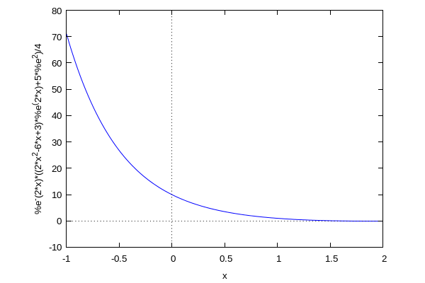
and shovels the conditions into x and y and solves for the integration constants. Let's do this again, but we will conclude by catching the final solution in a function sol(x):
| --> |
ode2('diff(y,x)+2·y = x^2 − 2·x,y,x); ic1(%,x=1,y=1); define(sol(x),rhs(%)); |
Now we are free to do whatever we want with sol(x) including differentiating it:
| --> | diff(sol(x),x); |
or graphing it:
| --> | wxplot2d(sol(x),[x,−1,2]); |
3.1 Second Order IVPs
Now let's use ic2() to apply initial conditions to second order IVPs. The syntax is
ic2([solution eqn], [indep var value], [dep var value], [dep var deriv val])
As an example, consider the damped spring IVP: x'' +3x' + 7x = e^t cos(2t), x(0)=1, x'(0)=1/2:
| --> |
ode2('diff(x,t,2)+3·'diff(x,t)+7·x=exp(t)·cos(2·t),x,t); ic2(%, t=0,x=1,'diff(x,t)=1/2); |
Please note the way that x'(0) = 1/2 is used in the command with the prime notation. This is really the only way to do this.
So for IVPs, the primed notation is really the only option.
Of course, we can chain and catch just as we had before. So let's expand the
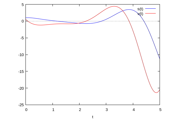
above so that we catch the final result in a function s(t):
| --> |
ode2('diff(x,t,2)+3·'diff(x,t)+7·x=exp(t)·cos(2·t),x,t)$ ic2(%,t=0,x=1,'diff(x,t)=1/2)$ define(s(t),rhs(%)); |
Note that the $ signs just supress the output of the lines that we aren't really
interested in. Now that we have s(t) -- the position function -- we could
graph it as well as graph its velocity as well!
| --> | wxplot2d([s(t),diff(s(t),t)],[t,0,5],[legend,"s(t)","v(t)"]); |
4 Boundary Conditions
Boundary conditions for second order equations are handled with the command bc2().
Note that there is no such thing as a boundary condition for a first order ODE (think
about this for a second). The syntax of bc2() is:
bc2(solution,[indep val 1],[dep val 1], [indep val 2], [indep val 2])
So let's solve the boundary value problem: x'' + x = t^3, x(0)=0, x(1)=5.
| --> |
ode2('diff(x,t,2)+x=t^3,x,t)$ bc2(%,t=0,x=0,t=1,x=5); |
And of course we could have caught the solution if we wanted to using define(soln(t),rhs(%)) as in previous examples. Let's do another:
| --> |
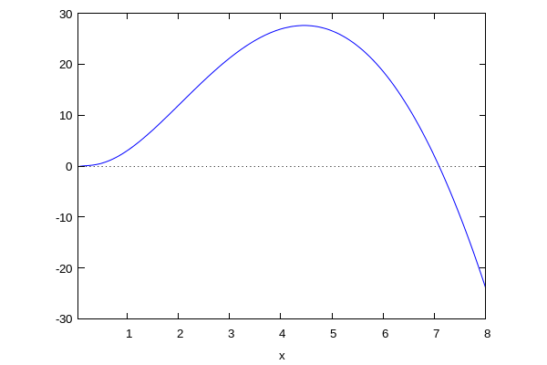
ode2(x^2·'diff(y,x,2)−3·x·'diff(y,x) + 5·y = cos(log(x)),y,x)$ bc2(%,x=1,y=3,x=7,y=2)$ define(f(x),rhs(%)); |
Just as an illustration, let's graph y=f(x) on the axes below to get a feel for the (admittedly), pretty awful solution above:
| --> | wxplot2d(f(x),[x,.05,8]); |
5 More Notation and Flexibility
To conclude, we remind ourselves that Maxima can bind any object, value, expression, equation to a symbol.
So, for example, we could bind a differential equation: y'' - 5y' + 9y = x^2 + x cos(3x) to the symbol EQN like
so:
| (%i8) | EQN: 'diff(y,x,2)−5·'diff(y,x) + 9·y = x^2 + x·cos(3·x); |
NOw, if we want to solve the above, we simply type:
| (%i9) | ode2(EQN,y,x); |
The beauty of the above is that it is clearly the same command that we could recycle
as we change the underlying equation. For example:
| (%i18) | EQN2: 'diff(y,x) − (1/x) · y = x; |
| (%i19) | ode2(EQN2,y,x); |
Not only does this allow us to conveniently recycle code, with this way of doing things, we can clearly see the differential equation in its symbolic form before we feed it to ode2() to solve. This allows us a convenient way
to troubleshoot any typos or mistakes on our part in a much friendlier way.
Let's use the above idea to solve the BVP: y'' + 1.23 y = cos(3.4x), x(0)=1, x(%pi/3.4)=2
| (%i20) | EQN3: 'diff(y,x,2) + 1.23·y = cos(3.4·x); |
| (%i22) |
ode2(EQN3,y,x); bc2(%,x=0,y=1,x=%pi/3.4,y=2); |
That last one is a bit agressive, so let's use a float() command to just make everything a decimal:
| (%i28) |
ode2(EQN3,y,x)$ bc2(%,x=0,y=1,x=%pi/3.4,y=2)$ define(soln(x),rhs(float(%))); |
| (%i29) | kill(all); |