Functions of Multiple Variables: Partial Derivatives and Total Differentials
1 Functions of Multiple Variables
First, we note that expressions in multiple variables can easily be bound to a variable as we have seen in the past:
| --> | E:x^2+y^2; |
| --> | E; |
To evaluate the above expression at x=1 and y=2 we can simply substitute:
| --> | subst([x=1,y=2],E); |
Of course, we don't need the intermediate step of defining E for this to work:
| --> | subst([x=1,y=2],x^2+y^2); |
It would be easier, however, if we had a function f(x,y) that could be called instead of an expression E.
We define such a function in the same way as a single variable function, using the := operator:
| --> | f(x,y):=x^2+y^2; |
And now, evaluation happens in the natural way:
| --> | f(1,2); |
As before, we can compose expressions into our functions:
| --> |
f(x,2*x+5); expand(f(x,2*x+5)); |
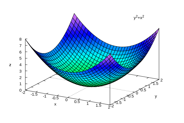
We can of course plot our functions too:
| --> | wxplot3d(f(x,y),[x,-2,2],[y,-2,2]); |
Functions of three or more variables are also possible. Take for example:
| --> | g(x,y,z):=x+y-cos(z); |
| --> | g(1,2,%pi/2); |
| --> | h(x):=sqrt(x[1]^2+x[2]^2+x[3]^2+x[4]^2); |
The above is used by treating x as a vector (list) and pulling out its first four elements:
| --> | h([a,b,c,d]); |
Let's clean up:
| --> | kill(all); |
2 Partial Derivatives
To get a partial derivative of a multi-variate function in Maxima, we simply use the derivative operator diff()
and specify which variable we would like to compute the partial with respect to. For instance:
| --> |
f(x,y):=2*x+3*y; 'diff(f(x,y),x)=diff(f(x,y),x); 'diff(f(x,y),y)=diff(f(x,y),y); |
As per usual, it is not necessary to pre-define a function for this to work:
| --> | 'diff(2*x+3*y,x)=diff(2*x+3*y,x); |
And we can also use the ev(,nouns) trick to make life a little clearer in displaying what we are computing alongside
the result of that computation:
First, we define the symbolic expressions we wouldl like to take:
| --> |
f(x,y,z):=2*x+3*y+4*z; fx:'diff(f(x,y,z),x); fy:'diff(f(x,y,z),y); fz:'diff(f(x,y,z),z); |
Then we crunch through the results:
| --> |
fx=ev(fx,nouns); fy=ev(fy,nouns); fz=ev(fz,nouns); |
Incidentally, we can use ev(,diff) to force the symbolic expression to evaluate as well:
| --> |
ev(fx,diff); ev(fy,diff); ev(fz,diff); |
2.1 Catching the Partial as a New Function
In order to *catch* the derivative and use it as a function in its own right, we must utilize the define() function:
| --> |
f(x,y,z):=exp(x^2+y^2+z^2); define(fx(x,y,z),diff(f(x,y,z),x)); |
Now fx is the x-partial derivative of f(x,y,z) that we can evaluate and use at will:
| --> | fx(1,0,2); |
2.2 Mixed Partials
We can compute mixed partials by simply stacking partial derivatives and taking multiple partial derivatives in a row. For example, if we wanted to compute all second order partials of f(x,y) = x^2+y^2 we would do:
| --> |
f(x,y):=x^2+y^2; define(fxx(x,y),diff(f(x,y),x,2)); /*Second order partial with respect to x only*/ define(fyy(x,y),diff(f(x,y),y,2)); /*Second order partial with respect to y only*/ define(fxy(x,y),diff(diff(f(x,y),x),y)); /*Mixed partial fxy*/ fyx(x,y):=fxy(x,y); /*Mixed partials are equal here.*/ |
| --> | kill(f); |
While the above works, it's a lot of writing. We can accomplish the same thing using the % tag and a few lines
of computation. Let's compute a partial fxyzz for the following function:
| --> | f(x,y,z):=(x^2+y^2)*exp(x^2+y^2+z^2); |
| --> | diff(f(x,y,z),x); |
| --> | diff(%,y); |
So we've computed fxy at this point, we will wrap it up by differentiating twice with respect to z and catching
the result as our finished product:
| --> | define(fxyzz(x,y,z),diff(%,z,2)); |
And now we have fxyzz at our disposal:
| --> | fxyzz(1,1,0);fxyzz(1,1,1);fxyzz(0,1,0); |
2.3 Chaining Partials for Clarity and Ease
Let's conclude by computing fxxyyzzz for a function f(x,y,z) that we can easily check the validity of, but we will do it all in one pass in sequence:
| --> |
f(x,y,z):=x^2*y^2*z^3; diff(f(x,y,z),x,2)$ diff(%,y,2)$ define(fxxyyzzz(x,y,z),diff(%,z,3)); |
The above is accomplished by "chaining" the partials one after another using the % symbol (that refers to the output of the last computation). Since all of the operations are grouped into a single block of commands, there is little danger of the % symbol
getting re-defined as we work through our other problems in our notebook.
Also note the use of $ signs versus the ; symbols. Recall that the $ signs suppress output, while the ; displays it.
Let's clean up:
| --> | kill(all); |
3 Total Differentials
The differential of a function f(x,y) is composed of the partials of f(x,y) , dx, and dy. We get it by using diff like so:
| --> |
f(x,y):=x^2+y^2; diff(f(x,y)); |
Notice the absence of the particular target variables x and y in the diff() command, and the symbols del(y) and del(x)
in the result. del(y) and del(x) are short for "dy" and "dx."
Let's take a few total differentials and catch the results:
| --> |
f(x,y):=x^2 + x*y^2; df:diff(f(x,y)); df2:diff(x^2+x*y^2); |
Now, if we want to evaluate df we simply substitute the values for the constituent parts like so:
| --> | subst([del(x)=.1,del(y)=-.2,x=1,y=1],df); |
The above is machine for: -0.1.
Note that we must be very careful about the order in which we substitute:
| --> | subst([x=1,y=1,del(x)=.1,del(y)=-.2],df); |
This is due to the fact that:
| --> | subst(x=1,del(x)); |
Once del(x) and del(y) have been altered to del(1), then del(x) and del(y) are no longer there to substitute for.
So the del() expressions must be dealt with FIRST.
3.1 Making the Differential Look "Right"
One way to get around the "wierdness" that we saw above with del(x) and del(y) and to make them easier to work with is to simply replace them with dx and dy and to define a new function in terms of x,y, dx, and dy like so:
| (%i11) |
f(x,y):=x^3*y^2*exp(x*y); /*Define the original function*/ diff(f(x,y)); /*Take the total differential of the function*/ subst([del(x)=dx,del(y)=dy],%); /*Replace del(x) and del(y) in the previous output*/ define(df(x,y,dx,dy),%); /*Define df(x,y,dx,dy) as the function given by the last output*/ |
Now we see that x and dx are independant of one another, as are y and dy.
The above requires more commands, but each command is simple, and the result is much clearer to use in practice.
Let's clean up and then do a serious example:
| (%i12) | kill(all); |
3.2 A Specific Example:
A sphere and a cylinder are welded together to give a volue of V(r,R,h) = %pi*r^2*h + (4/3)*%pi*R^3. Here
r is the radius of the cylinder, h is the height of the cylinder and R is the radius of the sphere. Let's compute
dV when r=2,R=3,h=4,dr=dh=dR=0.02.
| --> |
diff(%pi*r^2*h+(4/3)*%pi*R^3)$ subst([del(r)=dr,del(R)=dR,del(h)=dh],%)$ define(dV(r,R,h,dr,dR,dh),%); |
| --> | dV(2,3,4,0.02,0.02,0.02); |
Of course, if we are careful about the order we substitue, we could knock the last example out in one pass:
| --> |
subst([del(r)=.02,del(R)=.02,del(h)=.02,r=2,R=3,h=4], diff(%pi*r^2*h+(4/3)*%pi*R^3)); |
Which is machine for 1.12%pi. While the above can be accomplished in one line, the previous approach is
far preferable for readability and troubleshooting purposes.