Integration
1 Basic Integration
1.1 Indefinite Integrals
The command to preform both an indefinite and definite integral are the same in Maxima.
To preform an indefinite integral we use the integrate(f(x),x) command. Note that the
first input is the function that we wish to integrate, while the second is the variable of
integration.
| --> | integrate(x^2+2*x,x); |
In the following example, we define a function f(t), bind I to its antiderivative family,
and then have Maxima show us the results of the indefinite integral:
| --> |
f(t):=sqrt(1+exp(t)); I:'integrate(f(t),t); I=ev(I,nouns); |
| --> | kill(f); |
1.2 "Catching" the Antiderivative Family
Let's say that we want to integrate 2x+cos(x) and assign its antiderivatives to a new function f(x).
If we try:
| --> | f(x):=integrate(2*x+cos(x),x); |
Then there are two problems:
1. We don't have the integration constant
2. Watch what happens when we try to evaluate f(3):
| --> | f(3); |
The issue here is the same that we faced with the derivative. We have to catch the antiderivative.
We will also add in an integration constant while we are at it:
| --> | kill(f); |
| --> | define(f(x),integrate(2*x+cos(x),x)+C); |
| --> |
f(x); f(%pi/2); |
| --> | kill(all); |
Much better! Now we can move on to finding specific antiderivatives using Maxima's solving capabilities.
1.3 Finding Antiderivatives that Satisfy a Specific Condition
Let's say that we want to find the antiderivative f(x) of 2x + cos(x) that satisfies f(pi/2) = 3.
Here's how we would do that:
| --> | define(f(x), integrate(2*x+cos(x),x)+C); |
So the above f(x) has the integration constant included. Now we want to apply the condition f(pi/2)=3:
First, we set-up the equation for the initial condition:
| --> | E:f(%pi/2)=3; |
Then we solve it and catch the solution:
| --> | S:solve(E,C); |
Finally, we bind the solution to the constant C:
| --> | C:rhs(S[1]); |
So that now f(x) is given by:
| --> | f(x); |
| --> | kill(f,C); |
It is important that you kill C if you plan on using it for your integration constant again, otherwise
it will keep its constant value that you assigned above!
1.4 Streamlining the Process
Note that we do not have to to all of these steps separately. Infact, let's streamline
this process in the following problem: Let's find the antiderivative F(x) of f(x)=x^3 - 2x+7
that satisfies F(0)=3:
| --> | f(x):=x^3-2*x+7; define(F(x),C+integrate(f(x),x)); |
| --> | C:rhs(solve(F(0)=3,C)[1]); F(x); |
| --> | kill(C,f,F); |
Let's pull apart the statement:
C:rhs(solve(F(0)=3,C)[1]);
Recall that solve(EQN,var) solves the equation EQN for the variable var and reports the result as a
list of equations like so:
| --> | solve(x^2 = x, x); |
So, we type: solve(F(0)=3,C) to solve for the value of C that we want -- there is only one
solution in the list, so we take: solve(f(%pi/2)=3,C)[1], and we complete the process by re-binding
the value of C to the right-hand side of the solution equation. Let's do this a few more times.
1.5 Examples of Particular Solutions to Antiderivatives
Find the function f(x) with:
f'(x) = cos^2(x) ; f(%pi/3) = 2/3
| --> | define(f(x),integrate(cos(x)^2,x)+C); |
| --> | C:rhs(solve(f(%pi/3)=2/3,C)[1]); |
| --> | f(x); |
This is a little goofy-looking. Let's try to simplify it:
| --> | ratsimp(%); |
Not Bad!
Now let's try to find the function f(x) with f'(x)=sin(sqrt(x)) with f(1) = 0.
We begin by killing f and C because we want to use them again:
| --> | kill(f,C); |
| --> | define(f(x),integrate(sin(sqrt(x)),x)+C); |
| --> | C:rhs(solve(f(1)=0,C)[1]); |
| --> | f(x); |
| --> | kill(f,C); |
Nice! This problem would have been pretty tough without the help of Maxima!
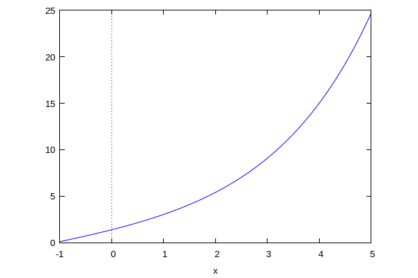
Let's find f(x) with: f'(x) = sqrt(1+%e^x) and f(0) = sqrt(2)
| --> | define(f(x), integrate(sqrt(1+exp(x)),x)+C); |
| --> | C:rhs(solve(f(0)=sqrt(2),C)[1]); |
| --> | f(x); |
The beauty of doing things this way is that now we can now go on to use f(x)
to find values, graph, etc:
| --> | f(0);f(log(2)); |
| --> | wxplot2d(f(x),[x,-1,5]); |
2 More than One Antiderivative
Let's say that I want the second antiderivative of x^2, call it f(x) that satisfies f(0)=1 and f'(0)=2.
Let's see what we can do here:
| --> | define(f(x),c[0]+integrate(c[1]+integrate(x^2,x),x)); |
Two things to note in the above:
1. To get two antiderivatives, we simply antiderived twice in succession, and
2. We used subscripts c[0], and c[1] to identify the integration constants.
Now let's solve for c[0] and c[1]:
| --> | C:solve([f(0)=1,subst(x=0,diff(f(x),x)=2)])[1]; |
Note that solve() always returns a list, and so to avoid a list-in-a-list situation, we simply ask for the list of solutions
with the index 1 above. Now we bind the solutions that we found to the constants:
| --> | c[1]:rhs(C[1]); c[0]:rhs(C[2]); |
| --> | f(x); |
Let's clean up!
| --> | kill(all); |
Let's repeat the exercise from above, but let's be a little more organized about it.
This time we will catch each antiderivative as it appears in its own function. Let's find the third antiderivative F(x) of
x*cos(x) that satisfies F(0)=1, F'(%pi)=2, and F''(%pi/2)=1.
| --> |
f[0](x):=x*cos(x); define(f[1](x),c[0]+integrate(f[0](x),x)); define(f[2](x),c[1]+integrate(f[1](x),x)); define(f[3](x),c[2]+integrate(f[2](x),x)); |
| --> | C:solve([f[3](0)=1,f[2](%pi)=2,f[1](%pi/2)=1])[1]; |
| --> | c[1]:rhs(C[1]);c[0]:rhs(C[2]);c[2]:rhs(C[3]); |
| --> | F(x):=f[3](x); |
| --> | F(x); |
The beauty of this is that now all three derivatives of F(x) are available in their entirety:
| --> | f[2](x);f[1](x);f[0](x); |
| --> | kill(all); |
3 Definite Integrals
The syntax for a definite integral is:
integrate(function,variable of integration, lower bound, upper bound)
To see this check out:
| --> | 'integrate(x^2,x,0,1); |
And as an example:
| --> |
I:'integrate(x^2,x,0,1); I=ev(I,nouns); |
Here are several more examples of definite integrals:
| --> |
I:'integrate(2^(2*x+1),x,-2,4); I=ev(I,nouns); |
| --> |
I:'integrate(cos(x)^4,x,0,%pi/4)$ I=ev(I,nouns); |
4 Improper Integrals at Infinity
When we want to compute improper integrals at ± infinity we use the bounds inf and minf respectively. So:
| (%i63) | I:'integrate(1/(x^2+1),x,minf,inf)$ I=ev(I,nouns); |
Or:
| (%i65) | I:'integrate(exp(-x^2),x,minf,0)$ I=ev(I,nouns); |
Or even still:
| (%i83) | I:'integrate(exp(-x),x,log(4),inf)$ I=ev(I,nouns); |
Wait... what?! Working with a CAS can sometimes be really frustrating. The above is correct, but what does it mean?
To get a better feeling, we try:
| (%i85) | float(rhs(%o83)); |
Oh... so it seems that the value is 1/4. This behavior is not uncommon for Maxima, Maple, or Mathematica and is just
one of the frustrations that we must deal with when allowing technology to do the heavy lifting for us.
5 Numerical Integration
Let's say we are not that interested in the symbolic value of a definite integral, but rather
the numberical value. Maxima has several methods of numerical integration. The most
useful and efficient is quad_qag(). quad_qag()??!! Let's give it a try to see how it works:
| (%i87) | quad_qags(cos(x)^4,x,0,%pi/4); |
quad_qags is a numerical method that uses approximating functions based on the technique of QUADrature to adaptively approximate the function so as to give a highly accurate approximation to the integral. Notice that the
result comes as a list with 4 elements. The first is the actual approximate value of the integral.
The second is the maximum error estimate. The third is information on the number of quadratic functions
used to approximate the curve, and the last element gives an ERROR type code.
We will be most interested in the first two elements in this list. If you just want the approximate value
of the integral, just ask for it:
| --> | quad_qags(cos(x)^4,x,0,%pi/4)[1]; |
If you want the error, ask for it as the second element in the list:
| --> | quad_qags(cos(x)^4,x,0,%pi/4)[2]; |
Of course, you could use float to approximate integrals:
| --> | float(integrate(cos(x)^4,x,0,1)); |
5.1 Numerical Integration and Infinite Bounds
If you want to find a numerical estimate of an integral with infinite boundaries, then you must use
a variant of quad_qags() called quad_qagi(). Here are some examples:
| (%i91) | 'integrate(exp(-x^2),x,2,inf)=quad_qagi(exp(-x^2),x,2,inf)[1]; |
| (%i93) | 'integrate(1/(x^2+sin(x)),x,minf,-2)=quad_qagi(1/(x^2+sin(x)),x,minf,-2)[1]; |
Note that quad_quagi() DOES NOT WORK ON FINITE INTERVALS!
| (%i96) | 'integrate(1/(x^2+sin(x)),x,-3,-2)=quad_qagi(1/(x^2+sin(x)),x,-3,-2)[1]; |
In which case we must use quad_qags():
| (%i97) | 'integrate(1/(x^2+sin(x)),x,-3,-2)=quad_qags(1/(x^2+sin(x)),x,-3,-2)[1]; |
Just for fun, let's try to compute the value of the above integral from -inf (minf) to inf (inf):
| (%i99) | 'integrate(1/(x^2+sin(x)),x,minf,inf)=quad_qagi(1/(x^2+sin(x)),x,minf,inf)[1]; |
Maxima sure did complain alot, but ultimately it gave us an answer. Unfortunately , the answer that it
gave is garbage! Error number 5 (when you read the manual for Maxima) is actually "integral is probably divergent..."
an indeed, this integral is divergent! Just because technology furnishes us with an answer does not mean we
should inherently trust it! To be fair, Maxima tried to let us know that this answer was extremely suspect!