Plotting in 3D with wxMaxima
As it turns out, there are several ways of making 3D plots in maxima.
We will only cover the wxdraw3d() [or draw3d()] methods that is found in the draw library.
The built in command wxplot3d() is quicker but can only plot surfaces of the form: z=f(x,y).
If we need to plot something like a sphere, a surface like x=g(y,z), or
a vector curve, then we will need to utilize the more flexible wxdraw3d()
function.
1 An Important Note about Style
Producing good looking 3D graphs in any computer algebra system
has as much to do with artistic choices as it does with the system's
power to compute. You may notice that a large portion of this tutorial
is committed to styling options and making choices to ensure that
the graphs that we produce "look good."
While asthetics are not typically the goal of making a graph --- we typically
make a graph to understand the general behavior of a function --- 3d graphs
can be complicated to the extent that if we do not put at least some effort
into how our graphs look they will ultimately be unreadable. An unreadable
graph can safely be put into the category of worthless.
2 Plotting with draw3d()
Maxima has an extensive graphing library for more advanced plots called draw. To gain access to it, we must load it in. To do this type in:
| --> | load(draw)$ |
Note that we ended the command with a $ sign. This is to suppress output.
During a load of draw, it is not uncommon Maxima to compile certain parts
of the draw package, and it may fill up the screen with compiling messages.
This should only happen the first time it is loaded on a machine, but if
Maxima has been updated, or if something has changed in the OS, it may
compile again. The messages can be safely ignored.
The command that comes with the draw package that we will focus on is wxdraw3d(). This command can be used to draw just about anything from points, to lines, to polygons, to contour maps, to surfaces --- It is an all purpose drawing command.
But because of this, it requires a little extra language to type in commands.
2.1 Plotting Surfaces z=f(x,y)
To plot a surface z=f(x,y), we use the syntax:
wxdraw3d(explicit(f(x,y), x, xmin, xmax,y,ymin,ymax))
Note that wxdraw3d() does not use brackets like wxplot3d() does. Everything
in wxdraw3d() is done via a list and keyword arguments.
| --> | wxdraw3d(explicit(x^2+y^2,x,-2,2,y,-2,2)); |
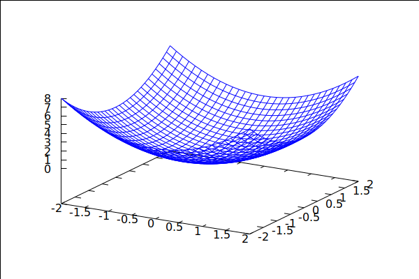
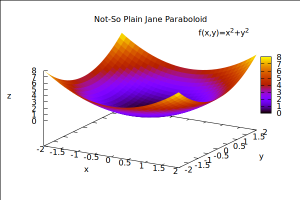
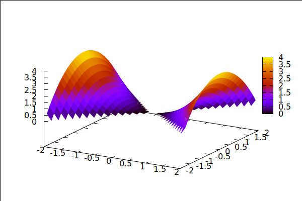
So the output here is a little barebones. If we want labels, legends, etc, we have to ask for them *before* we put in the function:
| --> |
wxdraw3d( enhanced3d=true, title="Not-So Plain Jane Paraboloid", xlabel="x", ylabel="y", zlabel="z", key="f(x,y)=x^2+y^2", explicit(x^2+y^2,x,-2,2,y,-2,2) ); |
If we don't want the color box on the side of the plot, or we don't care to see the axes, then we can turn them off with:
| --> |
wxdraw3d( enhanced3d=true, palette=[15,12,25], title="Fancy Nancy Paraboloid", key="f(x,y)=x^2+y^2", colorbox=false, axis_3d=false, explicit(x^2+y^2,x,-2,2,y,-2,2) ); |
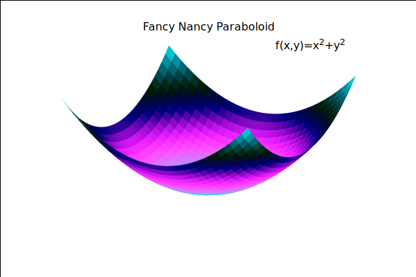
Notice that the palette was switched as well. The palette command will produce
a gradient based on the RGB values that you give it in the list.
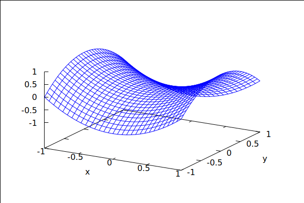
2.2 Changing the viewing angle
wxdraw3d() uses the view option to change teh viewing angle. Let's explore how it works with a hyperbolic paraboloid.
First, the paraboloid in its usual orientation:
| --> | wxdraw3d(explicit(x^2-y^2,x,-1,1,y,-1,1),xlabel="x",ylabel="y"); |
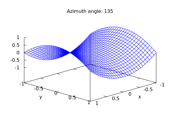
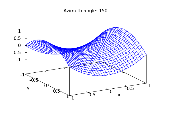
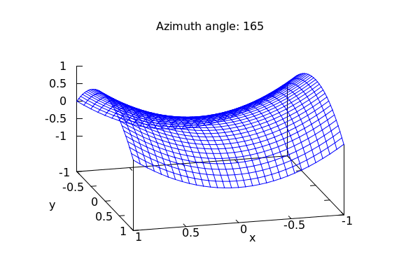
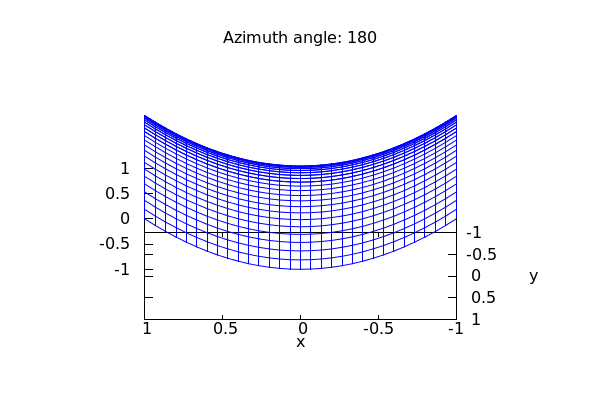
Now we look at the view option for several angles:
| --> |
for elevation:0 thru 90 step 15 do wxdraw3d(view=[elevation,0], title=concat("Elevation Angle: ",string(elevation)), explicit(x^2-y^2,x,-1,1,y,-1,1),xlabel="x",ylabel="y"); |
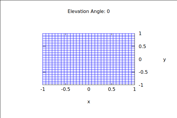
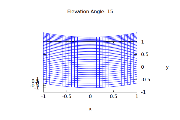
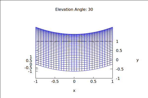
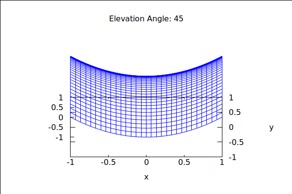
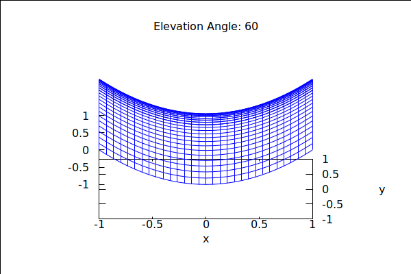
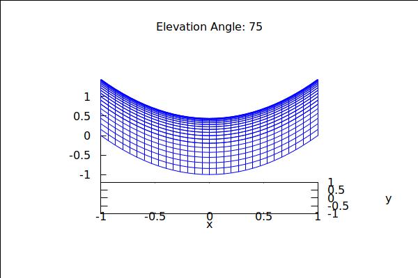
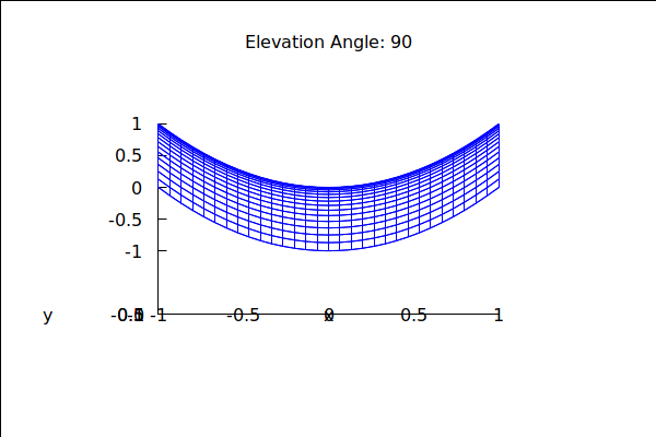
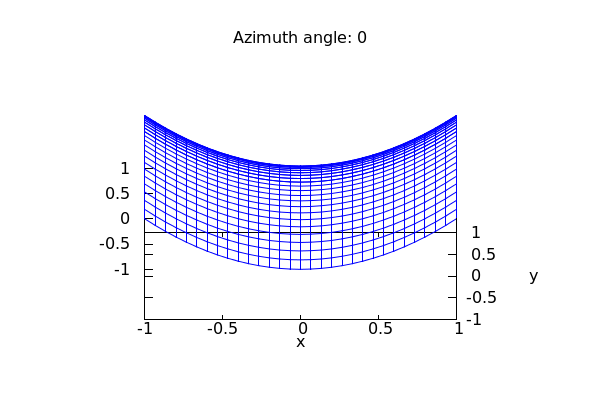
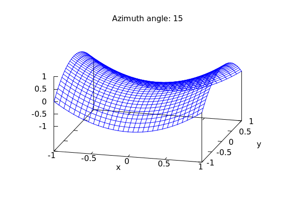
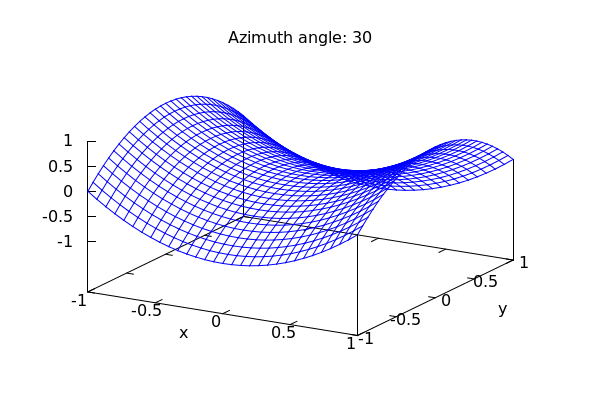
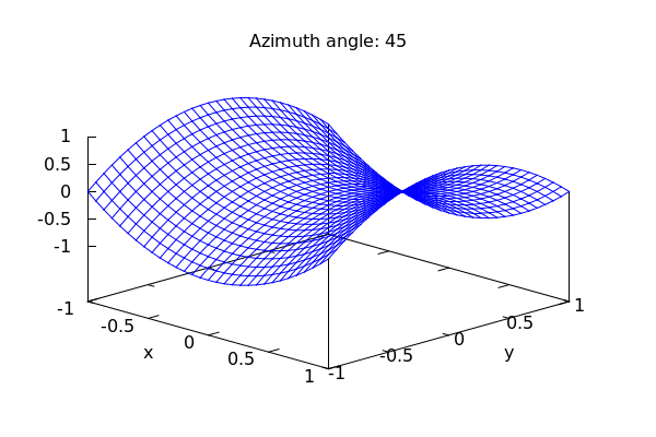
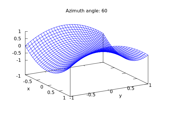
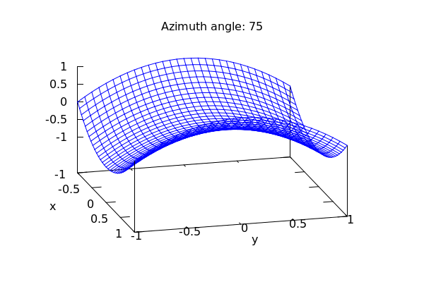
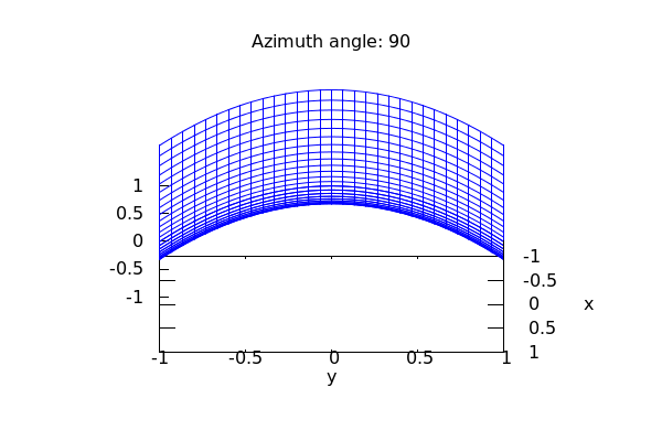
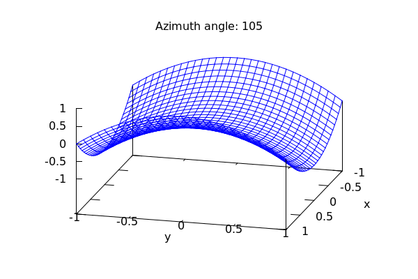
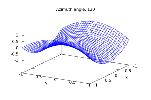
So in the view option, the first angle controls elevation. The second angle must control the rotation of the
xy-plane relative to the z-axis. Maxima calls this the azimuth angle. Let's explore:
| --> |
for azimuth:0 thru 180 step 15 do wxdraw3d(view=[60,azimuth], title=concat("Azimuth angle: ",azimuth), explicit(x^2-y^2,x,-1,1,y,-1,1),xlabel="x",ylabel="y"); |
2.3 A Caution about Axis Labels
If you look closely at the labeling of axes in the examples provided above, you will note that the labels for axes are placed at the outer-edge of the viewing box *along a line at a 90 degree angle to the direction of the axis.* This is fine if we leave that bounding box on, but it can cause serious problems if we turn it off and instead use the traditional axes that one finds in textbook drawings. We will see this issue in a few moments and we will have some thoughts on how to "hack" our way into the correct labels.
2.4 Last Thoughts on Explicit Surfaces with wxdraw3d()
Let's say that we want to see only the upper portion of: z = x^2-y^2. Then we can restrict
the range of the plot just as before:
| --> | wxdraw3d(enhanced3d=true,zrange=[0,4],explicit(x^2-y^2,x,-2,2,y,-2,2)); |
Notice that the above plot is a little blocky. We can up the resolution using the xu_grid and yv_grid options.
The defaults are around 30. So a value much higher will smooth things out considerably. CAUTION: setting
the number of gridlines higher will increase rendering times. On older machines, you may have to
wait a while!
| --> |
wxdraw3d( colorbox=false, palette=[15,5,20], title="One Good Looking Loid", enhanced3d=true, xu_grid=300, yv_grid=300, zrange=[-1,4], xlabel="x",ylabel="y",' xtics=none, ytics=none, explicit(x^2-y^2,x,-2,2,y,-2,2) ); |
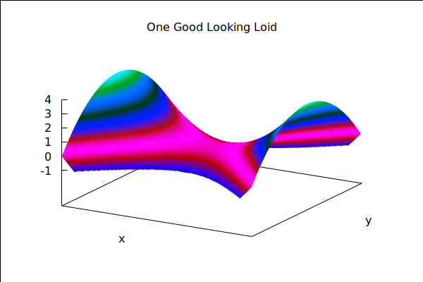
Note that we have used the options xtics=none and ytics=none to suppress the
labels on the x and y axes.
2.5 Multiple Plots, Aspect Ratios, xy-Plane, and Axes
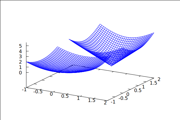
We can plot several surfaces in the same graph by defining them one at a time:
| --> |
S1:explicit(x^2+y^2,x,-1,1,y,-1,1); S2:explicit(4*sqrt((x-1)^2+(y-1)^2),x,0,2,y,0,2); wxdraw3d(S1,S2); |
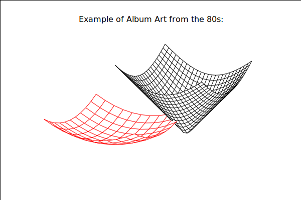
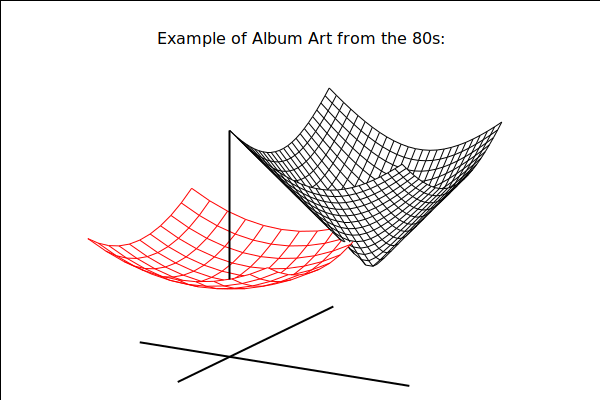
We can apply options to each graph as follows:
| --> |
wxdraw3d( title="Example of Album Art from the 80s:", surface_hide=true, color=red, xu_grid=10,yv_grid=10, S1, color=black, xu_grid=25,yv_grid=25, S2, axis_3d=false); |
It would be nice to see some axes in the above picture to orient ourselves, but we may not
want the fully labeled box that normally accompanies a plot. For this we use the (xyz)axis_type
option:
| --> |
wxdraw3d( title="Example of Album Art from the 80s:", surface_hide=true, xaxis=true,yaxis=true,zaxis=true, xaxis_type=solid,yaxis_type=solid,zaxis_type=solid, xaxis_width=2,zaxis_width=2,yaxis_width=2, color=red, xu_grid=10,yv_grid=10, S1, color=black, xu_grid=25,yv_grid=25, S2, axis_3d=false); |
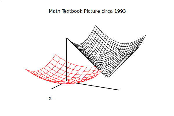
Ok, so why are the surfaces "floating" above the xy-plane? If you look at the original graphics box
you will note that the reference for the xy-plane was actually set at z=-5 or so. Let's force it to be
at z=0 to remove the "floating" effect:
| --> |
wxdraw3d( title="Math Textbook Picture circa 1993", surface_hide=true, xyplane=0, xlabel="x", xaxis=true,yaxis=true,zaxis=true, xaxis_type=solid,yaxis_type=solid,zaxis_type=solid, xaxis_width=2,zaxis_width=2,yaxis_width=2, color=red, xu_grid=10,yv_grid=10, S1, color=black, xu_grid=25,yv_grid=25, S2, axis_3d=false); |
Note the surface_hide=true option. This will hide any part of a surface obscured from view by any
other surface. Without it, both surfaces will show, potentially making the plot difficult to understand.
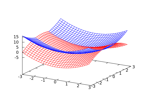
Here is an example where surface_hide is really useful:
| --> |
wxdraw3d( surface_hide=true, color=red, explicit(x^2-y^2,x,-3,3,y,-3,3), color=blue, explicit(x^2+y^2-2,x,-3,3,y,-3,3)); |
In addition to forcing the obscured surface to hide, we'll also give the graph a
legend as well as put in a typical set of axes into the picture.
| --> |
wxdraw3d( title="The Loid with Two Backs", view=[75,25], axis_3d=false, xaxis=true,yaxis=true,zaxis=true, xaxis_type=solid,zaxis_type=solid,yaxis_type=solid, xaxis_color=black,zaxis_color=black,yaxis_color=black, xaxis_width=3,yaxis_width=3,zaxis_width=3, xyplane=0, surface_hide=true, color=red, key="Hyperbolic Paraboloid", explicit(x^2-y^2,x,-4,4,y,-4,4), color=blue, key="Paraboloid", explicit(x^2+y^2-2,x,-4,4,y,-4,4) ); |
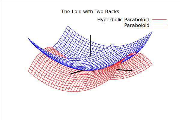
You may have noticed that the paraboloid doesn't quite look right -- It's not shaped
like a bowl like it should be. This is due to the fact that the x, y, and z axes are not
equal-measured. We can force the xy axes to have proportional scale as well as all
three axes using the proportional_axes option. Here we force x and y to have the same scale, which brings out
the "roundness" of the paraboloid:
| --> |
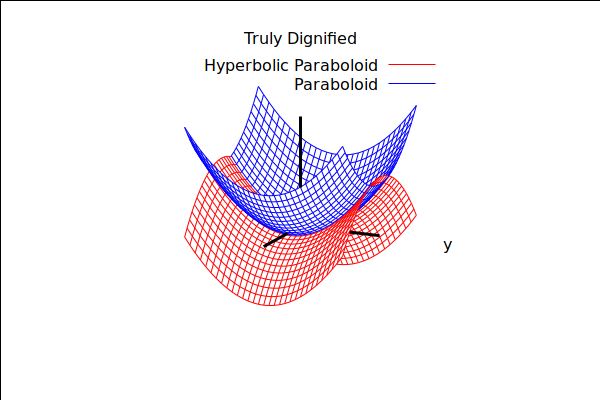
wxdraw3d( title="Truly Dignified", view=[75,25], proportional_axes=xy, axis_3d=false, xaxis=true,yaxis=true,zaxis=true, xaxis_type=solid,zaxis_type=solid,yaxis_type=solid, xaxis_color=black,zaxis_color=black,yaxis_color=black, xaxis_width=3,yaxis_width=3,zaxis_width=3, ylabel="y", xyplane=0, surface_hide=true, color=red, key="Hyperbolic Paraboloid", explicit(x^2-y^2,x,-4,4,y,-4,4), color=blue, key="Paraboloid", explicit(x^2+y^2-2,x,-4,4,y,-4,4) ); |
Finally, we note that you can generate an interactive window with your plot by leaving off
the wx in the wxdraw3d() commands and calling just draw3d().
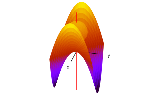
2.5.1 A Note about the Axis Label Placement
If you look carefully at the last example, you will see that the y-axis label appears to be in the right position,
but the hyperbolic paraboloid is opening in the wrong direction! Since z = x^2-y^2, it should be that the
parabolic cross sections parallel to the yz-plane are parabolas facing down, but the picture seems to be
showing that the cross sections parallel to the xz-plane are these downwards parabolas.
So what gives? If you go back and read section 3.3 you will recall that axis labels are not placed at the end of the axes, but
at a 90 degree angle to the axis. If we put the 3d-bounding box back into the last example, we can clearly see what's happening:
| --> |
wxdraw3d( title="Truly Dignified", view=[75,25], enhanced3d=false, proportional_axes=xy, axis_3d=true, /*We put the bounding box back into the picture*/ xaxis=true,yaxis=true,zaxis=true, xaxis_type=solid,zaxis_type=solid,yaxis_type=solid, xaxis_color=black,zaxis_color=black,yaxis_color=black, xaxis_width=3,yaxis_width=3,zaxis_width=3, ylabel="y", xyplane=0, surface_hide=true, color=red, key="Hyperbolic Paraboloid", explicit(x^2-y^2,x,-4,4,y,-4,4), color=blue, key="Paraboloid", explicit(x^2+y^2-2,x,-4,4,y,-4,4) ); |
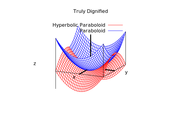
The y-axis is actually the line that is cutting toward the front of the picture since it is labeling at a 90 degree angle to that one,
while the x-axis is the line cutting through the opening of the hyperbolic paraboloid. So how do we fix this?! Well, since the labelling is occuring at 90 degrees to the actually lines, we can simply swap the x and y labels so that
xlabel="y", and ylabel="x"
And choose a viewpoint that places the correct axis as moving toward the front of the page:
| --> |
wxdraw3d( title="Truly Dignified", view=[60,105], /*We choose a view that places x in the front*/ enhanced3d=false, proportional_axes=xy, axis_3d=false, /*We remove the bounding box from the picture*/ xaxis=true,yaxis=true,zaxis=true, xaxis_type=solid,zaxis_type=solid,yaxis_type=solid, xaxis_color=black,zaxis_color=black,yaxis_color=black, xaxis_width=3,yaxis_width=3,zaxis_width=3, ylabel="x", /*We swap the labels*/ xlabel="y", xyplane=0, surface_hide=true, color=red, key="Hyperbolic Paraboloid", explicit(x^2-y^2,x,-4,4,y,-4,4), color=blue, key="Paraboloid", explicit(x^2+y^2-2,x,-4,4,y,-4,4) ); |
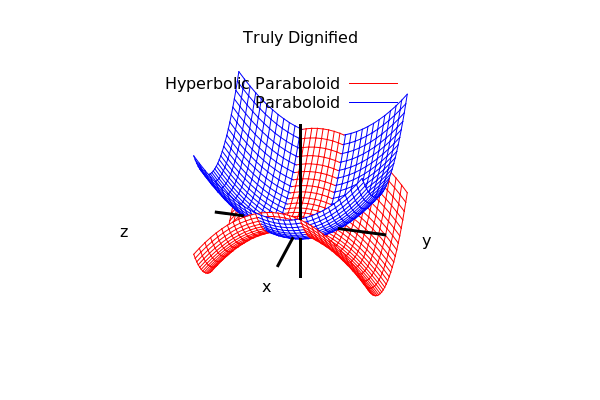
Much better! If you leave the bounding box on --- that is axis_3d=true --- this is entirely unnecessary, since it will be evident as to which axis belongs to which label. But if we toggle it off with axis_3d=false, we need to swap the labels and change our viewpoint. In what follows, the former is the approach that we will take since it aligns more closely with pictures that one finds in textbooks.
2.6 Implicit Surfaces
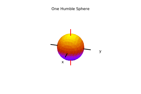
We can plot surfaces like spheres and ellipsoids using the implicit() option to wxdraw3d().
Note that proportional_axes command is going to be critical in a large number of these
plots, since the difference between an ellipsoid and a sphere, for instance,
comes down primarily to one of scale along the different axes!
| --> |
wxdraw3d( view=[60,105], xlabel="y",ylabel="x",zlabel="", title="One Humble Sphere", colorbox=false, axis_3d=false, xaxis=true,yaxis=true,zaxis=true, xaxis_type=solid,yaxis_type=solid,zaxis_type=solid, xaxis_width=3,yaxis_width=3,zaxis_width=3, xu_grid=300,yv_grid=300, enhanced3d=true, proportional_axes=xyz, xrange=[-3,3], yrange=[-3,3], zrange=[-3,3], implicit(x^2+y^2+z^2=4, x,-2,2, y,-2,2, z,-2,2) ); |
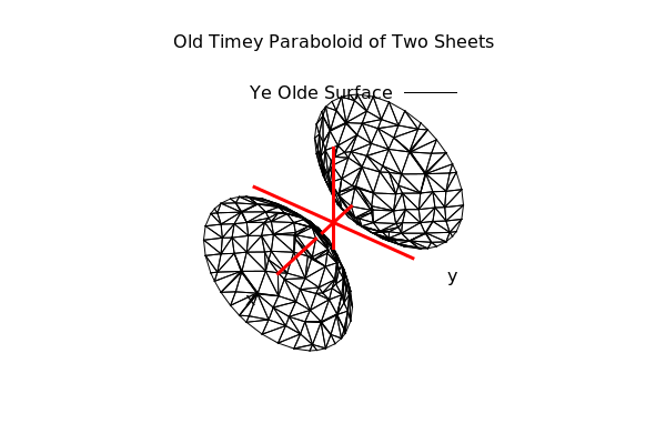
| --> |
wxdraw3d( view=[50,125], enhanced3d=false, title="Old Timey Paraboloid of Two Sheets", color=black, proportional_axes=xy, axis_3d=false, xaxis=true,yaxis=true,zaxis=true, xaxis_type=solid,yaxis_type=solid,zaxis_type=solid, xaxis_width=3,yaxis_width=3,zaxis_width=3, xaxis_color=red,yaxis_color=red,zaxis_color=red, xlabel="y", ylabel="x", zlabel="", xu_grid=50, key="Ye Olde Surface", implicit(y^2+z^2=x^2-1, x,-3,3, y,-3,3, z,-3,3) ); |
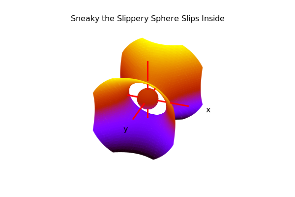
One more example. This example is much "smoother" looking than the others.
This is because we will increase the number of "cubes" (voxels) that the
plotting algorithm that wxdraw3d() uses to compute the surfaces. Beware!
Increasing the number of voxels past 20 will *dramatically* increase rendering
time. On older hardware, this could take upwards of 5 minutes to render!
| --> |
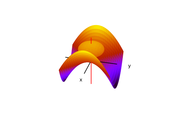
wxdraw3d( title="Sneaky the Slippery Sphere Slips Inside", xu_grid=200,yv_grid=200, x_voxel=40,y_voxel=40,z_voxel=40, proportional_axes=xy, enhanced3d=true, colorbox=false, axis_3d=false, xyplane=0, surface_hide=true, xaxis=true,yaxis=true,zaxis=true, xaxis_type=solid,yaxis_type=solid,zaxis_type=solid, xaxis_color=red,yaxis_color=red,zaxis_color=red, xaxis_width=3,yaxis_width=3,zaxis_width=3, ylabel="x",xlabel="y",zlabel="", implicit(x^2+z^2=y^2+1,x,-2,2,y,-2,2,z,-2,2), implicit(x^2+y^2+z^2=1/4,x,-1,1,y,-1,1,z,-2,2)); |
3 Settings and Defaults in draw3d():
You may have noticed that it takes *a lot* of typing to get a 3d graph to look decent. You may also have noticed that a lot of that typing is repeated from graph to graph.
A lot of this typing was actually unnecessary since once we set something in a graph, then all graphs after that will utilize those settings. So for instance, when we set the voxels to 40 in the example of the last section, any graph that we would produce after that would also have their voxels cranked to 40. This could be a good thing, or a disaster.
It would be nice if we could set the options that we wanted once --- in a clear and concise way --- and then have Maxima remember those options for us as defaults for each new graph that we draw. And then if we wanted to *override* those defaults, then we could easily do so. Luckily, the "draw" library has such a device. It is a function called:
set_draw_defaults()
And it does exactly what it claims. So if you are going to be making several plots all in the same style, it's probably a good idea to set your defaults first and then graph.
IMPORTANT NOTE: you can always override a default if you need to within the draw3d() and wxdraw3d() environment! Here is an example of some pretty decent defaults:
The first thing we are going to do here is to set the voxels back at a reasonable level:
| --> | set_draw_defaults(x_voxel=20,y_voxel=20,z_voxel=20); |
Now we will establish a decent set of defaults:
| --> |
set_draw_defaults( axis_3d=false, proportional_axes=xy, surface_hide=true, enhanced3d=true, colorbox=false, xaxis=true,yaxis=true,zaxis=true, xaxis_type=solid,yaxis_type=solid,zaxis_type=solid, xaxis_width=2,yaxis_width=2,zaxis_width=2, zaxis_color=red, xlabel="y",ylabel="x",zlabel="", xyplane=0, xtics=false,ytics=false,ztics=false, view=[60,105] ); |
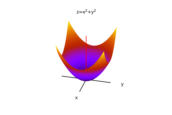
Now, any graph that we produce using wxdraw3d() or draw3d() will automatically employ these default values. Note also the swapped labels for x and y to line up with our custom "textbook" axes ends:
| --> |
wxdraw3d( title="z=x^2+y^2", explicit(x^2+y^2,x,-2,2,y,-2,2) ); |
| --> |
wxdraw3d( title="A Sphere and a Loid", explicit(x^2-y^2,x,-2,2,y,-2,2), implicit(x^2+y^2+(z-2)^2=1,x,-1,1,y,-1,1,z,1,3) ); |

Note that in the last example, the sphere is a little distorted because the axes are only proportional for x and y, not z.
We can force all three to be proportional by overriding the defaults that we set:
| --> |
wxdraw3d( proportional_axes=xyz, explicit(x^2-y^2,x,-2,2,y,-2,2), implicit(x^2+y^2+(z-2)^2=1,x,-1,1,y,-1,1,z,1,3) ); |
In this way the shape of the sphere is retained. Note that if we re-graphed the above without the proportional_axes=xyz,
we get:
| --> |
wxdraw3d( explicit(x^2-y^2,x,-2,2,y,-2,2), implicit(x^2+y^2+(z-2)^2=1,x,-1,1,y,-1,1,z,1,3) ); |
which is back to being squashed with disproportionate axes, because that is the default behavior of our graphs.
This is a much better way to handle graph options!